NAME
App::GUI::Cellgraph - draw pattern by cellular automata
SYNOPSIS
start the program (cellgraph)
push buttons and see patterns change
choose "Save" in Image menu (or
Ctrl+S) to store image in a PNG / JPEG / SVG file (choose image size in menu beforehand)choose Write in settings menu (
Ctrl+W) to save settings into an INI file for tweaking them later
DESCRIPTION
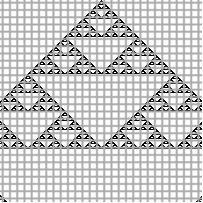
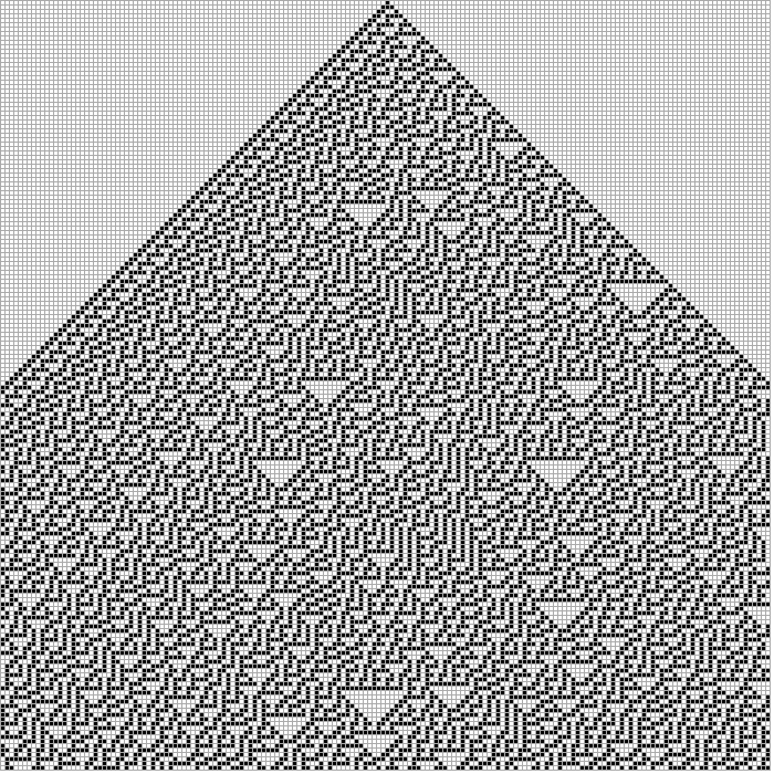
This is a row (one dimensional arrangement) of cellular automata. Their starting state can be seen as a color in the first row of the grid. Each subsequent row below reflects the following state (Y is time axis). Other drawing directions are optional and explained as part of the Global panel.


Mechanics
One automaton is called cell and works like described in Steve Wolframs book "A new kind of science". Each cell can be in one of several states, displayed as a greyscale or user defined color. The most simple cells have only two states: 0 and 1 (pictured as white and black squares). The state of each cell may change each round (think of processor cycles). How exactly they change is defined by a transfer function. The input of that function are the states of neighbours left and right and the cell itself. The size of this neighbourhood can be changed. For every combination of states in the neighbourhood there is one partial rule that defines the next state of the cell. If large neighbourhoods or large state counts would result in too many partial rules, than a different logic will apply. Than there is only a different partial rule for every distinct sum value. By sum is meant the sum of all states in the neighbourhood, since the state of a cell is just an integer.
To each partial rule also belongs also an action rule, an instruction that decides if the transfer function will be even applied or the state just stays the same. Action rules will be set via the Action panel.
GUI
The general layout is very simple: the settings are on the right and the drawing board is left. The settings are devided into several tabs.
Please mind the tool tips - short help texts which appear if the mouse stands still over a button. Also helpful are messages in the status bar at the bottom that appear while browsing the menu.
Global

The first tab contains the general (meta) settings. In upper left corder is the selector for the optical grid style. With or without grid lines (always sized one pixel) or just same sized gaps between the colored squares, which represent the cells. Right beside you set the size of the squares in pixel.
In the row below are options how to draw the state matrix. Default is the already in the description mentioned top down drawing method, where the first row is the initial state of the cells as set in the next tab named start. Each following state of a cell is in the square below, which makes Y so to speak the (vertical) time axis (top to down). To produce more decorative patterns there are two more frawing patters: inside out and outside in. Both are based on the idea of cutting the grid square into 4 triangles, by using the diagonals as dividing lines. With outside in the upper triangle is filled as before and the content rotated 3 times around the center to fill the other triangles. With the option inside out is almost everything the same except the upper triangle is filled from the center up so the central pixel of the square is the central pixel of the starting row, growing into all four directions. On the checkbox beside that you hab the option to make the leftmost and rightmost cells neighbours. It their not the program will calculate enough so no artefacts stemming from the corner cells will be visible. But making the cell row into a ring can produce a different kind of artefacts.
The third row in this tab sets the meta properties of the rules: number of states and size of neighbourhood. If that is even, the cell in question is not part of its own neighbourhood.
Start

The second tab contains settings for the starting values (states). By clicking on the squares you change (cycle) the state. Only the cells from the first to the last none zero (white) one will be recognised and placed into the center of the first grid row and the rest will be filled with zeros. If you choose Repeat, the selected cell staes will repeated to take up the entire cell row. To get only one none zero cell, press the butoon 1 and for a random starting sequence ?. The arrow buttons are just increment or decrement the numeric value of the starting sequence.
Rules

On the third tab you can set the individual partial rules. Just click on the result square in the chosen subrule (after the =>). The state color will cycle through as in the previous tab. All rule results are combined in a rule number, which you can see on top. With the buttons left and right you can again count that number down and up or even shift the rule results left and right (<< and >>). The buttons in the second row you to reach related rules, like the inverted, symmetric or opposite. Inverted means every sub rule result will be inverted. (Inverted result state, = $state_count - $previous_state ) Symmetric means every subrule switches its result with its symmetric partner (neighbourhood pattern or sum reversed). Opposite rule means the pattern of result states will be reversed (mirrored). The button "?" again selects a random rule.
Action

Here are listed the same sub rule inputs as before (every possible neighbourhood configuration) on the left hand side of the =>. The reults of these action rules control which cell are allowed to change during the next round (only neighbours marked with a circle). Behind the result of each subrule input is here a result for the action propagation. The circles show if the cell or its neighbours can do the transfer function next cycle. These settings are again combined in a singular action value (behind the label "Active:"). Here are also four buttons to select the init state, a grid patter or a random state. The first buttom set the inverted distribution of action propagation.
Menu
The upmost menu bar has only three very simple menus. Please not that each menu shows which key combination triggers the same command and while hovering over an menu item you see a short help text the left status bar field.
The first menu is for loading and storing setting files with arbitrary names. Also a sub menu allows a quick load of the recently used files. The first entry lets you reset the whole program to the starting state and the last is just to exit (safely with saving the configs).
The second menu has only two commands for saving the grin into a image file. It can have an arbitrary name - the ending PNG, JPG or SVG decides the format. The submenu above sets the image size. Please note that if you choose a larger image than shown, a larger grid will be computed. If you want larger squares, please change that in the settings.
SEE ALSO
AUTHOR
Herbert Breunung (lichtkind@cpan.org)
COPYRIGHT
Copyright(c) 2022 by Herbert Breunung
All rights reserved. This program is free software and can be used and distributed under the GPL 3 licence.