NAME
PDL::Graphics::Prima::DataSet - the way we think about data
SYNOPSIS
use PDL;
use PDL::Graphics::Prima::Simple;

my $x = sequence(100)/10 + 0.1;
my $y = $x->sin + $x->grandom / 10;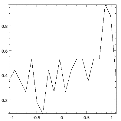
plot( -distribution => ds::Dist(
    $y, plotType => ppair::Lines,
    binning => bt::Linear,
));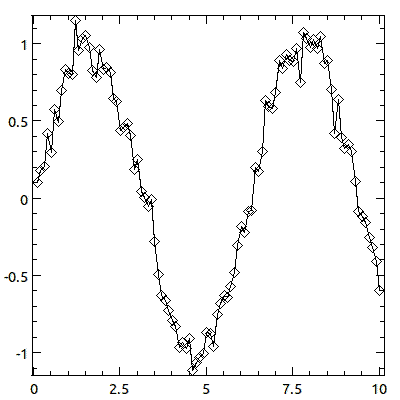
plot( -lines => ds::Pair(
    $x, $y, plotTypes => [ppair::Lines, ppair::Diamonds]
));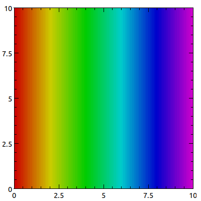
plot( -contour => ds::Grid(
    $x,
    bounds => [0,0,10,10],
    # Specify your bounds in one of these three ways
    # bounds => [$left, $bottom, $right, $top],
    # y_edges => $ys, x_edges => $xs,
    # x_bounds => [$left, $right], y_bounds => [$bottom, $top],
    # Unnecessary if you want the default palette
    plotType => pgrid::Matrix(palette => pal::RainbowSV(1.0, 0.8)),
));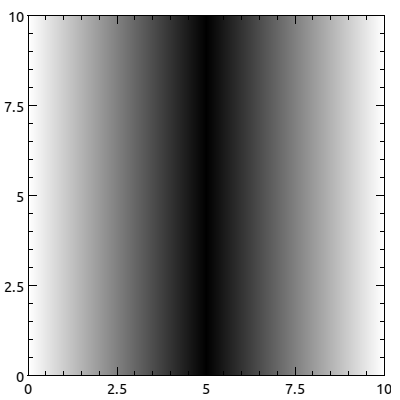
plot( -image => ds::Image(
    rvals(3, 256*2),
    format => 'string',
    # ... ds::Grid bounder options ...
    bounds => [0,0,10,10],
    # Unnecessary at the moment
    plotType => pimage::Basic,
));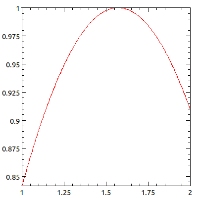
plot( -function => ds::Func( \&PDL::sin,
    color => cl::LightRed,
    xmin => 0, xmax => 1,
    N_points => 200,
));
DESCRIPTION
PDL::Graphics::Prima fundamentally conceives of two different kinds of data representations. There are pairwise representations, such as line plot used to visualize a time series, and there are gridded representations, such as raster images used to visualize heat maps (or images). Any data that you want to represent must have some way to conceive of itself as either pairwise or gridded.
Of course, there are plenty of things we want to visualize that are not pairwise data or grids. For example, what if we want to plot the distribution of scores on an exam? In this case, we would probably use a histogram. When you think about it, a histogram is just a pairwise visual representation. In other words, to visualize a distribution, we have to first map the distribution into a pairwise representation, and then choose an appropriate way to visualize that representation, in this case a histogram.
So, we have two fundamental ways to represent data, but many possible data sets. For pairwise representations, we have ds::Pair, the basic pairwise DataSet. ds::Dist is a derived DataSet which includes a binning specification that bins the distribution into bin centers (x) and heights (y) to get a pairwise representation. ds::Func is another derived DataSet that generates evenly sampled data based on the axis bounds and evaluates the supplied function at those points to get a pairwise representation. ds::Image provides a simple means for visualizing images, and ds::Grid provides a means for mapping a gridded collection of data into an image, using palettes.
Base Class
The Dataset base class provides a few methods that work for all datasets. These include accessing the associated widget and drawing the data.
- widget
-
The widget associated with the dataset.
- draw
-
Calls all of the drawing functions for each plotType of the dataSet. This also applies all the global drawing options (like
color, for example) that were supplied to the dataset. - compute_collated_min_max_for
-
This function is part of the collated min/max chain of function calls that leads to reasonable autoscaling. The Plot widget asks each dataSet to determine its collated min and max by calling this function, and this function simply agregates the collated min and max results from each of its plotTypes.
In general, you needn't worry about collated min and max calculations unless you are trying to grapple with the autoscaling system or are creating a new plotType.
working here - link to more complete documentation of the collation and autoscaling systems.
- new
-
This is the universal constructor that is called by the short-name constructors introduced below. This handles the uniform packaging of plotTypes (for example, allowing the user to say
plotType => ppair::Diamondsinstead of the more verboseplotTypes => [ppair::Diamonds]). In general, you (the user) will not need to invoke this constructor directly. - check_plot_types
-
Checks that the plotType(s) passed to the constructor or added at runtime are built on the data type tha we expect. Derived classes must specify their
plotType_base_classkey before calling this function. - init
-
Called by new to initialize the dataset. This function is called on the new dataset just before it is returned from
new.If you create a new dataSet, you should provide an
initfunction that performs the following:- supply a default plotType
-
If the user supplied something to either the
plotTypeorplotTypeskeys, thennewwill be sure you have you will already have that something in an array reference in$self->{plotTypes}. However, if they did not supply either key, you should supply a default. You should have something that looks like this:$self->{plotTypes} = [pset::CDF] unless exists $self->{plotTypes}; - check the plot types
-
After supplying a default plot type, you should check that the provided plot types are derived from the acceptable base plot type class. You would do this with code like this:
$self->check_plot_types(@{self->{plotTypes}});
This is your last step to validate or pre-calculate anything. For example, you must provide functions to return your data, and you should probably make guarantees about the kinds of data that such accessors return, such as the data always being a piddle. If that is the case, then it might not be a bad idea to say in your
initfunction something like this:$self->{data} = PDL::Core::topdl($self->{data}); - change_data
-
Sets the data to the given data by calling the derived class's
_change_datamethod. Unlike_change_data, this method also issues aChangeDatanotification to the widget. This means that you should only use this method once the dataset has been associated with a widget. Each class expects different arguments, so you should look at the class's documentation for details on what to send to the method. - compute_color_map_extrema
-
Multiple datasets and plot types can use the plot-wide color map. In that case, the color map needs to figure out the minimum and maximum values from the data. All datasets must run through their collection of plotTypes and ask each one for its color map extrema. PlotTypes should either return an empty list (indicating they are not using the plot-wide color map) or the lowest minimum value and the largest maximum value needed to render their data.
- has_custom_color_map
-
Returns true if the dataset has its own color map, false otherwise.
- color_map
-
Returns the color map of either the dataset or, if the dataset does not have a custom color map, the plot-wide color map.
Pair
Pairwise datasets are collections of paired x/y data. A typical Pair dataset is the sort of thing you would visualize with an x/y plot: a time series such as the series of high temperatures for each day in a month or the x- and y-coordinates of a bug walking across your desk. PDL::Graphics::Prima provides many ways of visualizing Pair datasets, as discussed under "Pair" in PDL::Graphics::Prima::PlotType.
The dimensions of pluralized properties (i.e. colors) should thread-match the dimensions of the data. An important exception to this is ppair::Lines, in which case you must specify how you want properties to thread.
The default plot type is ppair::Diamonds.
- ds::Pair - short-name constructor
-
ds::Pair($x_data, $y_data, option => value, ...)The short-name constructor to create pairwise datasets. The x- and y-data can be either piddles or array references (which will be converted to a piddle during initialization).
- expected_plot_class
-
Pair datasets expect plot type objects that are derived from
PDL::Graphics::Prima::PlotType::Pair. - get_xs, get_ys, get_data
-
Returns piddles with the x, y, or x-y data. The last function returns two piddles in a list.
- get_data_as_pixels
-
Uses the reals_to_pixels functions for the x- and y- axes to convert the values of the x- and y- data to actual pixel positions in the widget.
- change_data
-
Changes the data to the piddles passed in. For example,
$scatter_plot->dataSets->{'data'}->change_data($xs, $ys);
Distribution
Distributions are unordered collections of sample data. The typical use case of a distribution is that you have a population of things and you want to analyze their agregate properties. For example, you might be interested in the distribution of tree heights at your Christmas Tree Farm, or the distribution of your students' (or your classmates') test scores from the mid-term. Common ways for visualizing distributions are to plot their cumulative distribution functions or their histogram, but those are actually classic pairwise data visualization approaches. That means that what we really need are means for converting unordered sets of data into pairwise data. Distributions, therefore, let you specify the means by which your unordered data should be transformed into pairwise data, and the pairwise plot types to visualize the resulting transformed data. In an object oriented sense, the Distribution class is derived from the Pairwise class because a distribution is visualized using pairwise plot types.
Note that shape of pluralized properties (i.e. colors) should thread-match the shape of the data excluding the data's first dimension. That is, if I want to plot the cumulative distributions for three different batches using three different line colors, my data would have shape (N, 3) and my colors piddle would have shape (3).
PDL::Graphics::Prima's notion of distributions is not yet finalized and is open to suggestion. If you find yourself using distribution plots regularly, you should give me feedback on what works and what doesn't. Thanks!
- ds::Dist - short-name constructor
-
ds::Dist($data, option => value, ...)The short-name constructor to create distribtions. The data can be either a piddle of values or an array reference of values (which will be converted to a piddle during initialization).
In addition to the standard keys, there is also the
binningkey. Thebinningkey expects either a standard binning approach using one of the pre-defined forms, or a subroutine reference that performs the binning in a customized fashion. The binning types are all functions that expect key/value pairs that includeminandmaxfor the lower and upper threshold of the binning,drop_extremesto indicate if the data outside the min/max range should be included in the first and last bins, andnormalizeto indicate if the binning should be normalized to 1, for some appropriate definition of normalization. Other keys may also be allowed.If you want to write a customized binning function, it should accept the two arguments, the
datato bin and thedistributionobject. It should return a pair of piddles representing the x and y coordinates to plot. In addition, if the binning routine knows how to calculate properties for specific plot types, it can specify the plot type and any properties that it would provide for that plot type.For example, if you write a binning routine that knows how to calculate the bin boundaries for the Histogram plot type, your return statement could look like this:
return ($x, $y, Histogram => { binEdges => $bounds } );If your binning routine uses the number of points in a Symbols plot type to represent something, it could specify those:
return ($x, $y, Symbols => { N_points => $n_points } );If you have a means for calculating the error on your bins, you could include the error bar data:
return ($x, $y, ErrorBars => { y_err => $count_err } );These properties will be applied to the relevant plot types just before drawing and autoscaling operations, and any dataset operation that makes use of your supplied function should examine the additional parameters and act accordingly.
The standard binning types include:
- bt::CDF
-
Generates a cumulative distribution from the data. The default
minis the data's minimum, the defaultmaxis the data's maximum, the binning will notdrop_extremesby default (i.e.drop_extremes => 0) and the binning normalizes the data (i.e.normalize => 1). You can also specify if you want an increasing or decreasing representation by specifying a boolean value for theincreasingkey (the default is increasing, i.e. true).In the context of the CDF, normalization refers to the curve runnning from y = 0 to y = N - 1 (not normalized) or from y = 0 to y = 1 (normalized). Bear in mind that this interacts with your choice to drop the extremes or not.
In producing the CDF, bad values are simply skipped.
- bt::Linear
-
Generates a histogram from the data with linear spacing. The default
minis the data's minimum, the defaultmaxis the data's maximum, the binning willdrop_extremesby default (i.e.drop_extremes => 1) and the binning normalizes the data (i.e.normalize => 1). You can also specify the number of bins withnbins. The default is 20. If you want empty bins to be marked as bad, specifymark_empty_as => 'bad'. The default is to mark them as zero.In this case, normalization means that the "integral" of the histogram is 1, which means that the sum of the heights times the widths is 1.
- bt::Log
-
Generates a histogram from the data with logarithmic spacing. The default
minis the data's smallest positive value and the default max is the data's maximum value. If none of the data is positive, the binning type croaks. The binning willdrop_extremesby default (i.e.drop_extremes => 1) and the binning normalizes the data (i.e.normalize => 1). You can also specify the number of bins withnbins. The default is 20. If you want empty bins to be marked as bad, specifymark_empty_as => 'bad'. The default is to mark them as zero.As with linear binning, normalization means that the "integral" of the histogram is 1, which means that the sum of the heights times the widths is 1.
- bt::StrictLog
-
Identical to bt::Log, except that it croaks if it encounters any negative values. You can use this in place of bt::Log to sanity check your data.
- bt::NormFit
-
"Fits" the distribution between the specified min and max (defaults to the data's min and max) to a normal distribution. This bin type does not pay attention to the
drop_extremeskey, but it cares about thenormalizekey. If unspecified (the default), the curve will be scaled so that the area underneath it is the number of data points being fit. If normalized, the curve will be scaled so that the area under the curve will be 1. You can also specify the number of points to use in generating the curves by including theN_pointskey/value pair.I am pondering allowing the curve's min/max to take the current axis bounds min/max if the axes are not autoscaling. Thoughts appreciated.
- get_data, get_xs, get_ys
-
Returns the binned data, just the x-values, or just the y-values. For all of these, the binning function is applied to the current dataset. However, for the x- or y-getters, the other piece of data is discarded.
Grid
Grids are collections of data that is regularly ordered in two dimensions. Put differently, it is a structure in which the data is described by two indices. The analogous mathematical structure is a matrix and the analogous visual is an image. PDL::Graphics::Prima provides a few ways to visualize grids, as discussed under "Grids" in PDL::Graphics::Prima::PlotType. The default plot type is pgrid::Color.
This is the least well thought-out dataSet. As such, it may change in the future. All such changes will, hopefully, be backwards compatible.
At the moment, there is only one way to visualize grid data: pgrid::Matrix. Although I can conceive of a contour plot, it has yet to be implemented. As such, it is hard to specify the dimension requirements for dataset-wide properties. There are a few dataset-wide properties discussed in the constructor, however, so see them for some examples.
- ds::Grid - short-name constructor
-
ds::Grid($matrix, option => value, ...)The short-name constructor to create grids. The data should be a piddle of values or something which topdl can convert to a piddle (an array reference of array references).
The current cross-plot-type options include the bounds settings. You can either specify a
boundskey or one key from each column:x_bounds y_bounds x_centers y_centers x_edges y_edges- bounds
-
The value associated with the
boundskey is a four-element anonymous array:bounds => [$left, $bottom, $right, $top]The values can either be scalars or piddles that indicate the corners of the grid plotting area. If the latter, it is possible to thread over the bounds by having the shape of (say)
$leftthread-match the shape of your grid's data, excluding the first two dimensions. That is, if your$matrixhas a shape of (20, 30, 4, 5), the piddle for$leftcan have shapes of (1), (4), (4, 1), (1, 5), or (4, 5).At the moment, if you specify bounds, linear spacing from the min to the max is used. In the future, a new key may be introduced to allow you to specify the spacing as something besides linear.
- x_bounds, y_bounds
-
The values associated with
x_boundsandy_boundsare anonymous arrays with two elements containing the same sorts of data as theboundsarray. - x_centers, y_centers
-
The value associated with
x_centers(ory_centers) should be a piddle with increasing values of x (or y) that give the mid-points of the data. For example, if we have a matrix with shape (3, 4),x_centerswould have 3 elements andy_centerswould have 4 elements:------------------- y3 | d03 | d13 | d23 | ------------------- y2 | d02 | d12 | d22 | ------------------- y1 | d01 | d11 | d21 | ------------------- y0 | d00 | d10 | d20 | ------------------- x0 x1 x2Some plot types may require the edges. In that case, if there is more than one point, the plot guesses the scaling of the spacing between points (choosing between logarithmic or linear) and appropriate bounds for the given scaling are calculated using interpolation and extrapolation. The plot will croak if there is only one point (in which case interpolation is not possible). If the spacing for your grid is neither linear nor logarithmic, you should explicitly specify the edges, as discussed next.
At the moment, the guess work assumes that all the scalings for a given Grid dataset are either linear or logarithmic, even though it's possible to mix the scaling using threading. (It's hard to do that by accident, so if that last bit seems confusing, then you probably don't need to worry about tripping on it.) Also, I would like for the plot to croak if the scaling does not appear to be either linear or logarithmic, but that is not yet implemented.
- x_edges, y_edges
-
The value associated with
x_edges(ory_edges) should be a piddle with increasing values of x (or y) that give the boundary edges of data. For example, if we have a matrix with shape (3, 4),x_edgeswould have 3 + 1 = 4 elements andy_edgeswould have 4 + 1 = 5 elements:y4 ------------------- | d03 | d13 | d23 | y3 ------------------- | d02 | d12 | d22 | y2 ------------------- | d01 | d11 | d21 | y1 ------------------- | d00 | d10 | d20 | y0 ------------------- x0 x1 x2 x3Some plot types may require the data centers. In that case, if there are only two edges, a linear interpolation is used. If there are more than two points, the plot will try to guess the spacing, choosing between linear and logarithmic, and use the appropriate interpolation.
The note above about regarding guess work for x_centers and y_centers applies here, also.
- expected_plot_class
-
Grids expect plot type objects that are derived from
PDL::Graphics::Prima::PlotType::Grid. - get_data
-
Returns the piddle containing the data.
- change_data
-
Changes the data to the piddle passed in. For example,
$map_plot->dataSets->{'intensity'}->change_data($new_intensity); - guess_scaling_for
-
Takes a piddle and tries to guess the scaling from the spacing. Returns a string indicating the scaling, either "linear" or "log", as well as the spacing term.
working here - clarify that last bit with an example
Image
Images are like Grids (they are derived from Grids, actually) but they have a specified color format. Since they have a color format, this means that they need to hold information for different aspects of each color, so they typically have one more dimension than Grids. That is, where a grid might have dimensions M x N, an rgb or hsv image would have dimensions 3 x M x N.
The default image format is rgb. Currently supported image formats are rgb (red-green-blue), hsv (hugh-saturation-value), and prima (Prima's internal color format, which is a packed form of rgb).
As Images are derived from Grids, any method you can call on a Grid you can also call on an Image. Differences and details specific to Images include:
- ds::Image - short-name constructor
-
ds::Image($image, option => value, ...)Creates an Image dataset. A particularly important key is the
color_formatkey, which indicates the format of the$imagepiddle. When it comes to drawing the image, the data will be converted to a set of Prima colors, which means that the first dimension will be reduced away. Values associated with keys should be thread-compatible with the dimensions starting from the second dimension, so if your image has dims 3 x M x N, values associated with your various keys should be thread-compatible with an M x N piddle.Note that color formats are case insensitive. At the moment there is no way to add new color formats, but you should expect a color format API to come at some point in the not-distant future. It will very likely make use of PDL::Graphics::ColorSpace, so if you want your own special color format to be used for Images, you should contribute to that project.
- change_data
-
Sets the image to the new image data. Expects a piddle with the new data and an optional format specification. If no specification is given, the current format is used.
Func
PDL::Graphics::Prima provides a special pair dataset that takes a function reference instead of a set of data. The function should take a piddle of x-values as input and compute and return the y-values. You can specify the number of data points by supplying
N_points => valuein the list of key-value pairs that initialize the dataset. Most of the functionality is inherited from PDL::Graphics::Prima::DataSet::Pair, but there are a few exceptions.
- ds::Func - short-name constructor
-
ds::Func($subroutine, option => value, ...)The short-name constructor to create function datasets. The subroutine must be a reference to a subroutine, or an anonymous sub. For example,
# Reference to a subroutine, # PDL's exponential function: ds::Func (\&PDL::exp) # Using an anonymous subroutine: ds::Func ( sub { my $xs = shift; return $xs->exp; }) - change_data
-
Sets the function and/or the number of points to evaluate. The basic usage looks like this:
$plot->dataSets->{'curve'}->change_data(\&some_func, $N_points);Either of the arguments can be undefined if you want to change only the other. That means that you can change the function without changing the number of evaluation points like this:
$plot->dataSets->{'curve'}->change_data(\&some_func);and you can change the number of evaluation points without changing the function like this:
$plot->dataSets->{'curve'}->change_data(undef, $N_points); - get_xs, get_ys
-
These functions override the default Pair behavior by generating the x-data and using that to compute the y-data. The x-data is uniformly sampled according to the x-axis scaling.
- compute_collated_min_max_for
-
This function is supposed to provide information for autoscaling. This is a sensible thing to do for the the y-values of functions, but it makes no situation with the x-values since these are taken from the x-axis min and max already.
This could be smarter, methinks, so please give me your ideas if you have them. :-)
Annotation
PDL::Graphics::Prima provides a generic annotation dataset that is used for adding drawn or textual annotations to your plots.
- ds::Note - short-name constructor for annotations
-
ds::Note(plotType, plotType, ..., drawing => option, drawing => option)The short-name constructor to create annotations. This expects a list of annotation plot types fullowed by a list of general drawing options, such as line width or color. For example,
ds::Note(
    pnote::Region(
        # args here
    ),
    pnote::Text('text',
        # args here
    ),
    ... more note objects ...
    # Dataset drawing options
    color => cl::LightRed,
    ...
);
Unlike other dataset short-form constructors, you do not need to specify the plotTypes key explicitly, though if you did it would do what you mean. That is, the previous example would give identical results as this:
ds::Note(
    plotTypes => [
        pnote::Region(
            # args here
        ),
        pnote::Text('text',
            # args here
        ),
        ... more note objects ...
    ],
    # Dataset drawing options
    color => cl::LightRed,
    ...
);
The former is simply offered as a convenience for this more long-winded form.
DataSet::Collection
The dataset collection is the thing that actually holds the datasets in the plot widget object. The Collection is a tied hash, so you access all of its data members as if they were hash elements. However, it does some double-checking for you behind the scenes to make sure that whenever you add a dataset to the Collection, that you added a real DataSet object and not some arbitrary thing.
working here - this needs to be clarified
RESPONSIBILITIES
The datasets and the dataset collection have a number of responsibilities, and a number of things for whch they are not responsible.
The dataset container is responsible for:
- knowing the plot widget
-
The container always maintains knowledge of the plot widget to which it belongs. Put a bit differently, a dataset container cannot belong to multiple plot widgets (at least, not at the moment).
- informing datasets of their container and plot widget
-
When a dataset is added to a dataset collection, the collection is responsible for informing the dataset of the plot object and the dataset collection to which the dataset belongs.
Datasets themselves are responsible for:
- knowing and managing the plotTypes
-
The datasets are responsible for maintaining the list of plotTypes that are to be applied to their data.
- knowing per-dataset properties
-
Drawing properties can be specified on a per-dataset scope. The dataset is responsible for maintaining a list of these properties and providing them to the plot types when they perform drawing operations.
- knowing the dataset container and the plot widget
-
All datasets know the dataset container and the plot widget to which they belong. Although they could retrieve the widget through a method on the container, the
- informing plotTyes' plot widget
-
The plot types all know the widget (and dataset) to which they belong, and it is the
- managing the drawing operations of plotTypes
-
Although datasets themselves do not need to draw anything, they do call the drawing operations of the different plot types that they contain.
- knowing and supplying the data
-
A key responsibility for the dataSets is holding the data that are drawn by the plot types. Althrough the plot types may hold specialized data, the dataset holds the actual data the underlies the plot types and provides a specific interface for the plot types to access that data.
On the other hand, datasets are not responsible for knowing or doing any of the following:
- knowing axes
-
The plot object is responsible for knowing the x- and y-axis objects. However, if the axis system is changed to allow for multiple x- and y-axes, then this burden will shift to the dataset as it will need to know which axis to use when performing data <-> pixel conversions.
TODO
Add optional bounds to function-based DataSets.
Captitalization for plotType, etc.
Use PDL documentation conventions for signatures, ref, etc.
Additional datset, a two-tone grid. Imagine that you want to overlay the population density of a country and the average rainfall (at the granularity of counties, let's say). You could use the intensity of the red channel to indicate population and the intensity of blue to indicate rainfall. Highly populated areas with low rainfall would be bright red, while highly populated areas with high rainfall would be purple, and low populated areas with high rainfall would be blue. The color scale would be indicated with a square with a color gradient (rather than a horizontal or vertical bar with a color gradient, as in a normal ColorGrid). Anyway, this differs from a normal grid dataset because it would require two datasets, one for each tone.
AUTHOR
David Mertens (dcmertens.perl@gmail.com)
ADDITIONAL MODULES
Here is the full list of modules in this distribution:
- PDL::Graphics::Prima
-
Defines the Plot widget for use in Prima applications
- PDL::Graphics::Prima::Axis
-
Specifies the behavior of axes (but not the scaling)
- PDL::Graphics::Prima::DataSet
-
Specifies the behavior of DataSets
- PDL::Graphics::Prima::Limits
-
Defines the lm:: namespace
- PDL::Graphics::Prima::Palette
-
Specifies a collection of different color palettes
- PDL::Graphics::Prima::PlotType
-
Defines the different ways to visualize your data
- PDL::Graphics::Prima::ReadLine
-
Encapsulates all interaction with the Term::ReadLine family of modules.
- PDL::Graphics::Prima::Scaling
-
Specifies different kinds of scaling, including linear and logarithmic
- PDL::Graphics::Prima::Simple
-
Defines a number of useful functions for generating simple and not-so-simple plots
- PDL::Graphics::Prima::SizeSpec
-
Compute pixel distances from meaningful units
LICENSE AND COPYRIGHT
Unless otherwise stated, all contributions in code and documentation are copyright (c) their respective authors, all rights reserved.
Portions of this module's code are copyright (c) 2011 The Board of Trustees at the University of Illinois.
Portions of this module's code are copyright (c) 2011-2013 Northwestern University.
Portions of this module's code are copyright (c) 2013-2014 Dickinson College.
This module's documentation is copyright (c) 2011-2014 David Mertens.
This module is free software; you can redistribute it and/or modify it under the same terms as Perl itself.